Convolutional Neural Networks

Visual Perception

The same image perceived through different visual systems will result in perceptions suitable for their respective survival environments.

Different observation angles determine the recognition result of an image.

Image Representation

The input $x$ for image recognition is a three-dimensional tensor with shape (width, height, depth). Each (width, height) matrix is called a channel.

Image invariance: The position of an object in a channel should not affect the recognition result of that object.

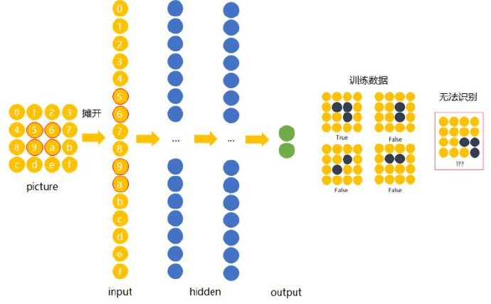
Why can’t feedforward neural networks complete this task?

The input image is a three-dimensional tensor, but obviously feedforward neural networks have difficulty recognizing “identical” samples at different positions. That is: feedforward neural networks should be able to recognize objects in images even when the objects are at different positions.

The most basic operations of convolutional neural networks:

Convolution
Non-linearity (ReLu)
Pooling
Classification (fully connected layer)

Convolution

Use local regions to scan the entire image

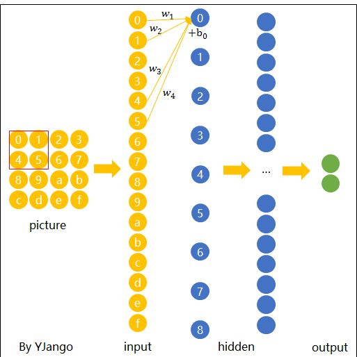
Where: the red box represents a filter or kernel, and hidden layer nodes are linear combinations of the kernel. Then, the expression for hidden layer node $y_0$ is: $$ y_0=x_0w_1+x_1w_2+x4w_3+x_5w_4+b_0 $$

Spatial sharing Different regions share the same “weight matrix” and bias $b_0$.

Matrix form output expression:

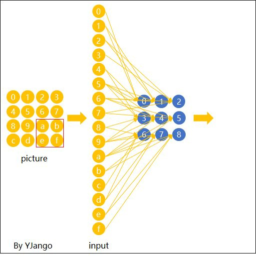
After one feature detector pass, the hidden layer can be viewed as “convolutional” features.

Processing the Depth dimension: Treat the three channels as three groups of different weight matrices Specifically, for a $$ 2\cdot2\cdot3 $$ (RGB) kernel, we have:

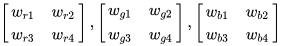
That is, the depth dimension is processed in a penetrating manner. In practice, the value of Depth is the same as the number of filters.

Stride: This parameter determines the number of pixels the filter slides over at once. In the examples in this article, the stride is all 1.

Zero padding To ensure the image size remains unchanged after convolution, padding with 0s on the outermost layer is needed.

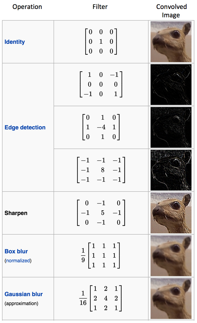
Multiple filters Different filters will capture different Feature Maps from the same image. Each different filter represents a different operation. The figure below shows different processing results of filters on the same image.

Non-linearity (ReLu)

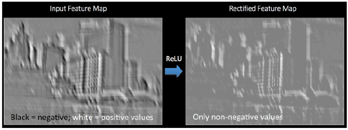
Let’s revisit our old friend ReLU: Rectified Linear Unit

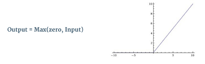
The main function of this stage is to set all pixels with negative values to 0.

Pooling

Max pooling The entire image is divided into several non-overlapping blocks of the same size (pooling size). Only the maximum number in each small block is taken, and after discarding other nodes, the output is obtained while maintaining the original planar structure. So why have this stage?

There is redundant information in the Feature Map after convolution that is unnecessary for object recognition.

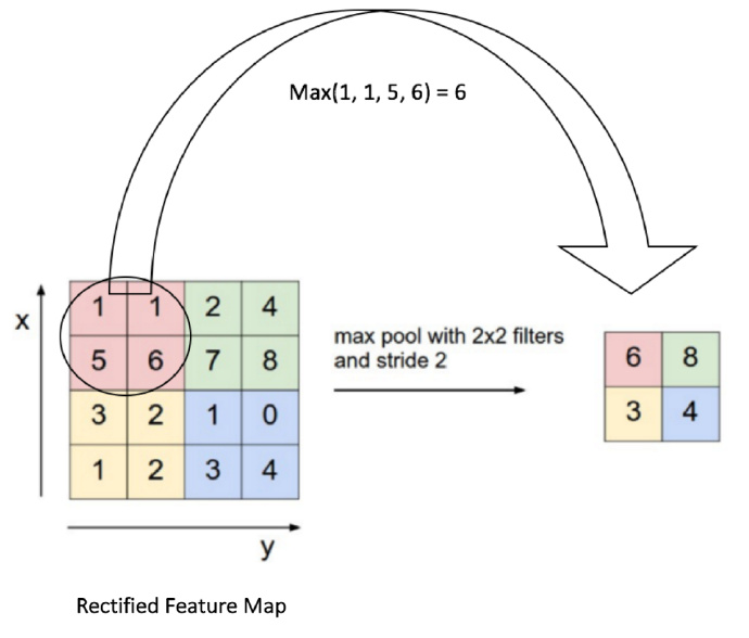
Note: The stride in the above diagram is set to 1

Fully Connected Layer

At the end of a convolutional network, the resulting cuboid is flattened into a long vector and fed into the fully connected layer along with the output layer for classification.

Summary: Training process of convolutional neural networks

Randomly initialize all filters, parameters, and weights
Use training images as input and go through the process of convolution -> ReLu -> pooling -> fully connected layer to find the probability of each classification.
Calculate the total error at the output layer.
Use gradient descent backpropagation to update the values of all filters, parameters, and weights. Weights are updated proportionally to the error they contribute.

Another example to fill in the gaps

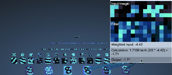
Visualize CNN game, strongly recommended to try!

Game screenshot is as follows: An image consists of 1024 ($32*32$) pixels.

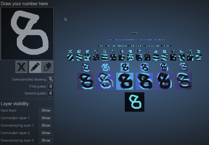
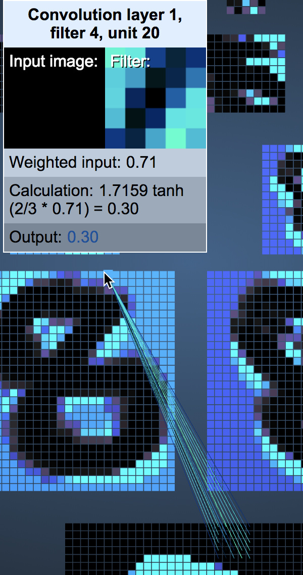
The first convolutional layer is generated by 6 $5*5$ filters with stride set to 1. We can vividly understand its depth dimension as 6. Note: The following diagram combines the ReLu stage and the convolution stage. Readers should be aware of this.

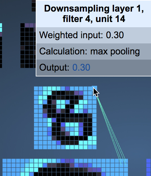
Next, use $2*2$ max pooling with stride 2 for each feature map. You can see that each pixel in the Pooling layer corresponds to four pixels in the Conv layer.

Next is the most difficult part to understand: the second convolution layer and max pooling layer. First, observe the number from the first max pooling layer to the second convolutional layer. Why do 8 feature maps become 16 feature maps after passing through filter f convolution?

To find the answer, let’s look at what the filters of the second layer feature maps look like:

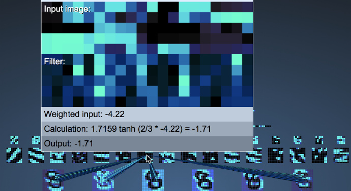
Please observe the above diagram carefully: We will find that the shape of the filters in the second convolutional layer is closely related to the selected feature map of the first max pooling layer! That is, when we do the second layer convolution, we only examine the local features of the first layer!

The second layer max pooling is the same as the first layer, so I won’t elaborate further.

Then comes the fully connected layer, which utilizes all features: