Introducing Computational Graphs
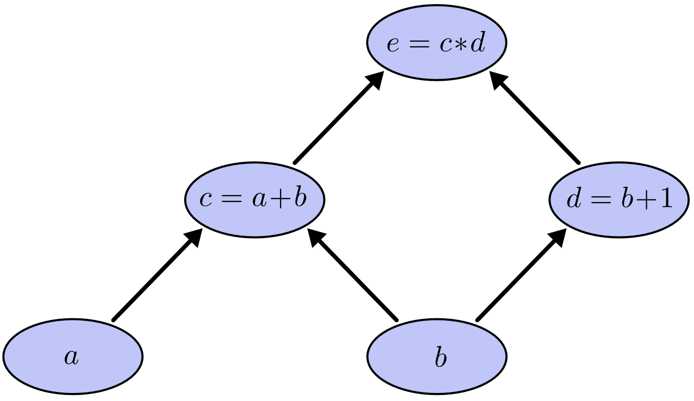
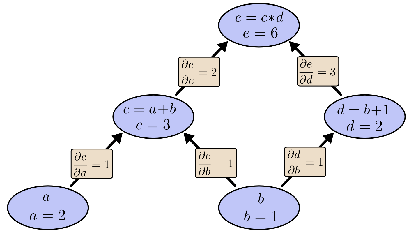
The following computational graph represents $e=(a+b)(b+1)$. We can assign values to node $a$ and node $b$ to calculate $e$
Factoring Path
Consider the chain rule for the following diagram:
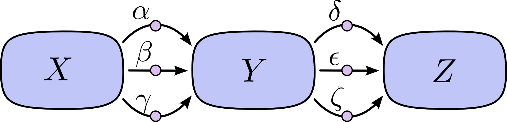
If we want to calculate $\frac{\partial Z}{\partial X}$, we must calculate $3*3=9$ paths:
$$ \frac{\partial Z}{\partial X} = \alpha\delta + \alpha\epsilon + \alpha\zeta + \beta\delta + \beta\epsilon + \beta\zeta + \gamma\delta + \gamma\epsilon + \gamma\zeta (1) $$
Factoring the above equation, we have:
$$ \frac{\partial Z}{\partial X} = (\alpha + \beta + \gamma)(\delta + \epsilon + \zeta) (2) $$
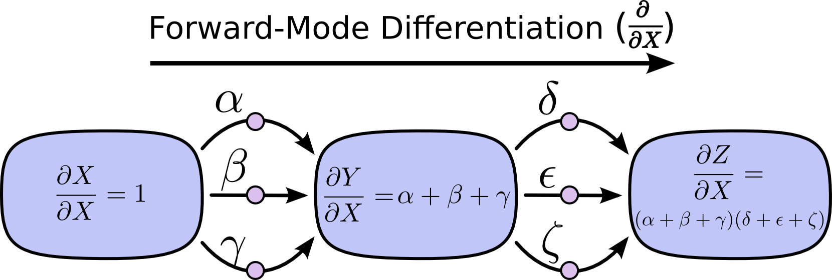
Equation (2) leads to “forward-mode differentiation” and “reverse-mode differentiation”: both efficiently compute partial derivatives through factorization.
Forward-mode Differentiation
By summing the inputs of paths on each node, we can obtain the partial derivative of how each input “influences” the node on the total path.
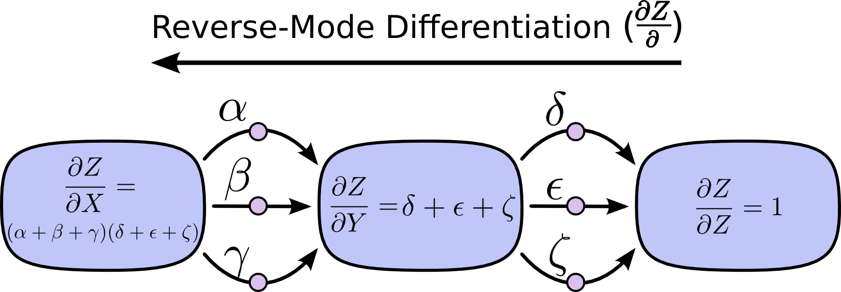
Reverse-mode Differentiation
Starting from the output node of the computational graph, move towards the initial node and merge all paths emanating from that node at each node:
Comparison of Forward-mode and Reverse-mode Differentiation
-
Forward-mode differentiation: tracks how each input affects all nodes, requires computing $\frac{\partial}{\partial X}$ for each node.
-
Reverse-mode differentiation: tracks how all nodes affect one output, requires computing $\frac{\partial Z}{\partial}$ for each node.
Speed Improvement in Computation
If we add partial derivatives to each edge of the computational graph, we have:
When we use forward-mode differentiation to compute the partial derivative of each node with respect to $b$:
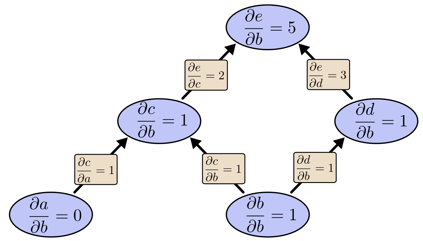
As shown in the diagram above, the cost of computing $\frac{\partial e}{\partial b}$ is that we need to compute many “useless” partial derivatives. [Note: “useless” because in the gradient descent process, we only care about the partial derivative of the output with respect to each node]
When we use reverse-mode differentiation to compute the partial derivatives of $e$ with respect to each node:
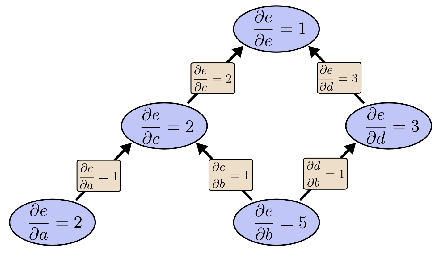
Comparing the two diagrams, we can find that reverse-mode differentiation “truly” gives us the partial derivatives we want. In extreme cases with millions of inputs, forward-mode differentiation needs to compute millions of times to get the partial derivatives of the output result with respect to all nodes. While reverse-mode differentiation only needs to compute once. When we train neural networks, we need to compute partial derivatives with respect to all parameters for gradient descent, so reverse-mode differentiation greatly improves computational speed.
Once you’ve framed the question, the hardest work is already done
References and citations: https://colah.github.io/posts/2015-08-Backprop/